

Red States And Blue States, The Missing Ingredient In Most Campaigns
- Brainz Magazine

- Feb 11, 2023
- 12 min read
Written by: Oren M. Levin-Waldman, Political Consultant, Labor Economist and Data Analyst, PoliticalVIP
The 2022 midterm election will go down as historical because the President’s party did not lose a large number of seats in Congress. The red wave that pollsters and pundits promised never really materialized. The Republicans eked out a narrow victory in the House of Representatives, but did not gain control of the Senate. This can be explained by a couple of forces that professionals in the field missed. First of all, pollsters got this election wrong, as they have been wrong on the last few dating at least to the 2016 election. Asking respondents how they feel about inflation and rising energy costs, is not the same as serious data about underlying transformations of which inflation and rising energy costs are merely symptoms. Democrats no doubt overplayed their hand on the narrative of how MAGA Republicans threaten our democracy, especially when they weren’t addressing the major policy concerns of the electorate. Similarly, Republicans underestimated the impact of the Supreme Court’s decision overturning Roe v. Wade. Although they focused on rising prices and rising crime, they offered little to counteract the Democrat claim that they opposed “our democracy.” Economic transformations that have left many ordinary workers, especially blue-collar in manufacturing, displaced and feeling neglected by political elites were not addressed. And yet, data shows that it is because of these voters’ concerns that Donald Trump was elected president in 2016.

In this article, I argue that traditional polling data is limited and that campaign managers who fail to do a deep dive into data on demographics, i.e., educational attainment, industry and occupational composition, etc. and which identify changing economic trends, may not be providing sufficient information to their candidates so that they can adequately identify and articulate the issues. Although public opinion polling may be useful, it could be fine tuned on the basis of information from demographic profiles. I argue that it is the inattention to this information that is precisely why the Democrats lost the 2016 presidential election, and ultimately why Republicans didn’t do as well as they were projected to. At the same time, the data suggest that the polarization plaguing the country is really a tale of two economies.
Data
It has been customary to divide the country into blue states and red states. Red states are primarily Republican and tend to be more conservative while blue states are primarily Democrat and tend to be more liberal. This would, of course, suggest that the divisions in the country are ideological, and peripherally this may be so. The data, however, suggest serious economic differences between them. It has been commonplace to break down demographics along gender, race and ethnic lines, as well as educational attainment and age. For the purposes of this analysis, the critical demographics are those of the labor markets, i.e., industrial and occupational, along with educational attainment. Data for this part is drawn from the IPUMS Current Population Survey (CPS) for the years 2008, and 2016. I specifically look at those workers between the ages of 18 and 65 who are working full-time.
When states are divided along these lines, we can see some clear differences between them in their respective labor markets. Because the focus is on those full-time workers working for wages, I am only looking at wage inequality, rather than the larger category of household wealth and income inequality. Table 1 shows levels of wage inequality according to 90/10, 90/50 and 50/10 percentile ratios and the top-to-bottom quintile ratios.
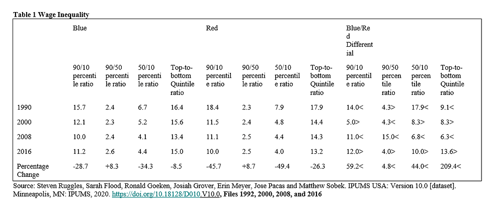
Wage inequality decreases in both blue and red states, but the decrease is greater in red states than in blue states, which also means that in 1990 there was greater inequality in red states. In 1990 and 2008, there is greater wage inequality in red states on all measures except the 90/50 percentile measure in 1990. But in 2000 and 2016, there is greater wage inequality in the blue states on all measures except the 90/50 percentile than in red states. On all measures, except the 90/50 measure, wage inequality decreased in both blue states and red states, but more so in red states between 1990 and 2016. On the 90/50 percentile measure, wage inequality increased 4.8 percent more in red states than in blue states between 1990 and 2016. On the top-to-bottom quintile ratio, wage inequality in red states decreased by 26.3 percent whereas it only decreased by 8.5 percent in blue states, a difference of 209.4 percent. That wage inequality decreases more in red states that in blue states between 1990 and 2016, may be suggestive of a widening gap between the top and the bottom particularly in blue states.
The question that needs to be addressed is whether there is a difference in industrial and occupational composition between red states and blue states, as well as educational attainment, that might account for less of a decrease in wage inequality in blue states than in red states. Michael Lind (2020) has suggested that American society could best be divided into the managerial elites who are well educated and employed in higher paying occupations, and everybody else. Everybody else would be considered ordinary workers, many of whom do not possess an abundance of skills. The managerial elites, which he sometimes refers to as the managerial overclass, are technocrats who also believe in a global economy. Most of this group are highly educated workers armed with university educations, and many are doing quite well in the financial and high-tech sectors, which also include information technology. This is the group that has discretionary income to spend on luxury goods, and this is the group that exercises considerable influence over the political leadership. That is, these are affluent voters that the political class tends to be more responsive to (Bartels 2008).
It would be useful here to group workers on the basis of occupational groups that approximate Lind’s classification: Professional/Manager, Skilled, Unskilled, and Other. Both skilled and unskilled refer primarily blue-collar workers. By this grouping, we can see some interesting differences in inequality. But also grouping the Professionals and Managers into the Professional/Manager group, we may have a demographic that approximates the money-manager. Professional/Managers would include those in the professions; those working in Finance and Real Estate; Management executives; and those working in Information and Technology. Those working in Skilled blue-collar jobs would include those working as Craftsmen and Operatives while those working as Unskilled blue-collar would include those classified as Laborers.
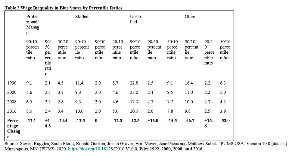
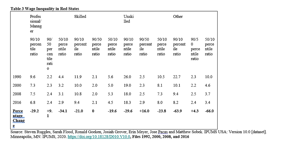
In 1990, there was still greater wage inequality in red states than in blue states. On the basis of this grouping, we can see that there have been greater decreases in wage inequality in red states than in blue. Despite declines in wage inequality income inequality has nonetheless increased, which can be accounted for by the fact that the two really aren’t the same. Wages are the income workers receive from work. Income, however, includes wages, plus dividend income and interest for those at the top, and in-kind assistance and other social supports for those at the bottom. Greater wage inequality in blue states, however, may have something to do with more skilled workers at the top in blue states and more unskilled workers at the bottom, whereas in red states there may be more of a middle, although it too appears to be dwindling. The question, then, is whether workers with certain demographic characteristics, labor market and otherwise, are more likely to be in blue states than in red states. A logistical regression analysis can help sort that out. Because the CPS data is individual level data, it will only tell us that individual workers with certain characteristics are either more or less likely to be in either a blue or red state. Therefore, two regressions are done, with being a blue state as the dependent variable in the first regression, and being a red state as the dependent variable in the second regression.
The objective is to present a contrast between blue and red states. The logistical regression involves dichotomous variables set at either 0 or 1. By setting variables to either 0 or 1 we should see that whatever the effects of the independent variables are on the dependent variable of being in a blue state will be the opposite of the effects of the same independent variables on the dependent variable of being in a red state. As the coefficients show this is mostly true, but they are not exactly opposites. By showing two regressions, the objective is to demonstrate just how different blue states are from red states. It makes sense, then, to look at skilled blue-collar workers as an independent variable. Skilled workers combine the occupational categories of craftsmen and operatives, and are most likely among the higher paying blue collar jobs. Manufacturing and Mining are also independent variables because they are better paying industries and may well speak to significant differences between red states and blue states. Finance and Real Estate is an important variables because that is where we are more likely to find those who can be classified as money managers; it too is an independent variable. Educational attainment is important because it speaks to a degree of skills to the extent that it serves as a proxy for skills. It is also important because members of the managerial class are more likely to have advanced degrees. Therefore, it is an independent variable too. But a High School Degree as the highest level of educational attainment is also an independent variable because it speaks to a more blue-collar economy. Business and Repair services is an important variable as well as Services are important because they both speak to a more service-oriented economy. In some cases more skills will be required, and in other cases their absence, or less of a presence, may speak to a more traditional industrial production economy. Lastly, as we have already observed, blue states have greater wage inequality, whether one lives in a state where there is greater wage inequality than in the U.S. as a whole becomes an important independent variable as well. Regression coefficients and their statistical significance can be seen in Table 4 and 5.
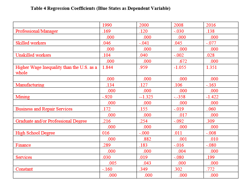
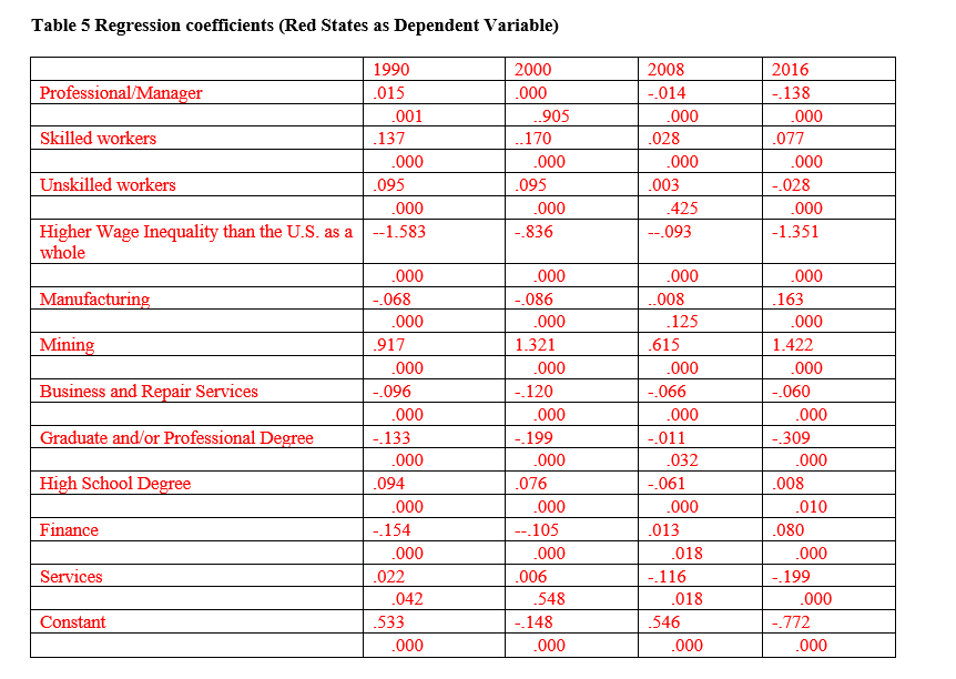
We find that in 1990 and 2016, those living in states where wage inequality is higher than the nation as a whole are also more likely to be in blue states. That is, they are less likely to be in red states, which is suggestive that there is less wage inequality in red states than in blue states., which is to say that there is also less wage inequality in red states. This may speak to blue states having more workers at the top and bottom of the distribution, with fewer in between. This may account for why wage inequality is higher in blue states, and would support the proposition that wage inequality has been about the top pulling away from everybody else (Stiglitz 2012; Pikkety 2014). The ranks of the top appear to be greater in blue states than in red states. Moreover, because there is less dispersion in red states, red states may not see inequality as the problem that blue states do.
The regression coefficients would appear to confirm a tale of two economies. For the exception of 2008, those with advanced degrees are more likely to be found in blue states, and less likely to be found in red states. This is an important variable for a couple of reasons. First, it is a proxy for skills, albeit it isn’t a perfect one. Second, advanced university awarded degrees speak to the presence of a managerial/professional class. And that the coefficient becomes stronger over time may speak to the growth of this managerial/professional class of which money managers are members. At the same time, having a high school diploma as the highest level of educational attainment is not statistically significant in blue states in 2000 and 2008, and the effects are small in the other years, almost as though it is a given that most people have a minimum of a High School degree. And yet, a High School degree as the highest level of educational attainment appears to be more significant in red states, which might be suggestive that workers have more opportunities with only a high school education in red states than they do in blue states. The change of the coefficient in blue states and its decrease in size in red states may reflect what Goldin and Katz (2008) refer to as the decline of the high school premium as a contributing factor to rising inequality.
Working as a Professional/Manager has positive effects for being in a blue state, but is either not statistically significant or negative in red states. Working in Finance and Real Estate has strong positive effects in 1990 and 2000 but either has little effect or a negative effect in 2008 and 2016 in blue states; so its effect weakens by 2016. In red states it is negative, but begins to have a slight effect by 2008 and 2016 Working in services, which would include information technology, however, has little effect for being in a blue state but by2016 it does have a relatively stronger effect, whereas in the red state it has little effect in 1990 and 2000 but becomes negative by 2008 and 2016. For the exception of 2008, being a blue-collar skilled worker has negative effects for being in a blue state. Also for the exception of 2008, being an unskilled worker has a small positive effect for being in a blue state. In red states, however, it is positive beginning in 1990, but its effect does weaken by 2016. Working in Manufacturing has a positive effect for being in a blue state beginning in 1990, but becomes negative in 2016, which may speak to a greater decline in manufacturing in blue states than in red states, whereas its effects for being a red state are small, and even negative in 2008. It does become positive by 2016, which may suggest that despite its overall decline in the country it is still more of a presence in red states than in blue states. What has a positive effect, for the exception of 2008, is working in Business and Repair Services in blue states. In red states, however, it is negative throughout. This too may represent an industry where more skilled workers are needed. Or here are where there are opportunities for skilled blue-collar workers.
We have already noted demographic differences along with differences in wage inequality. But differences in inequality will most likely have something to do with differences in their respective wage structures. Historically the overall wage structure was always lower in the South than it was in the North (Schulman 1990). Median and mean wages are also considerably higher in blue states than in red states. Of course, this will have something to do with the higher cost of living in those states. Still, differences in wage structure can create a prism through which workers in particular states view a wide range of issues.
Conclusion
Demographic profiles of these states confirmed that in these three states in particular that there had been a tremendous loss in the manufacturing base. Generally, states that flipped from blue to red in the 2016 election did so because of the changes in the economy. That is, the loss of manufacturing effectively left behind large numbers of workers who felt the global economy, and by extension decades of economic policymaking, left them behind. There was little statistical support for the idea that voters were responding to an increase in undocumented workers. On the contrary, the presence of Mexican workers in red states appeared to have absolutely no significance. Of course, the other issue that received little discussion in the last election was rising inequality, which continues to be an issue today. Rising inequality, of course, isn’t responsible for the changing base of the economy. Rather the changing base of the economy is reflected in rising income inequality. The two are very much interrelated. If the changing base of the economy can be said to be responsible for greater polarization, as data from the CPS suggests, then by extension we can conclude that increased polarization in the U.S. is also a function of rising income inequality.
Of course, none of this fits the convenient narrative that those who voted for Trump did so because they are racist. Rather they voted for him because they felt all but neglected by the other party advocating that they get used to working in new industries And yet, since the Democratic party has had no answers for the economic transformations responsible for the displacement of many workers, if not for the disappearance of the middle class, it has opted for the politics of diversion or what has come to be known as identity politics.
Ultimately, this should lead to the conclusion that serious campaign strategy requires more analysis along the lines presented in this article. Although public opinion polling has its place, much of what they really need to know in order to craft a message is already contained in the demographics of respective labor markets. If labor market profiles tell us that the economy has changed and how it has changed, can we draw implications for serious policy proposals? Surely this would be more meaningful than simply proposals based on simply opinion polling.

Written by: Oren M. Levin-Waldman, Political Consultant, Labor Economist and Data Analyst
Oren M. Levin-Waldman is a VIP Specialist at PoliticalVIP. As a Labor Economist and Former Professor, Levin-Waldman has served at prestigious universities like Rutgers University, Newark and New School University in New York.
Levin-Waldman’s expertise includes demographic and economic data analytics, labor economics, voting behavior statistics and researching. Just a few publications authored by Levin-Waldman are listed here:
References:
Goldin, Claudia and Lawrence F. Katz. 2008. The Race Between Education and Technology. Cambridge, MA: Belknap Press of Harvard University Press.
Levin-Waldman, Oren M. Restoring the Middle Class Through Wage Policy: Arguments for a Minimum Wage. London and New York: Palgrave Macmillan.
Meltzer, Alan H. and Scott F. Richard. 1981. “A Rational Theory of the Size of Government.” Journal of Political Economy. 89,5: 914-927.
Ruggles, Steven, Sarah Flood, Ronald Goeken, Josiah Grover, Erin Meyer, Jose Pacas and Matthew Sobek. 2019. IPUMS USA: Version 9.0 [dataset]. Minneapolis, MN: IPUMS,. https://doi.org/10.18128/D010.V9.0. Files for 2008 and 2016.


